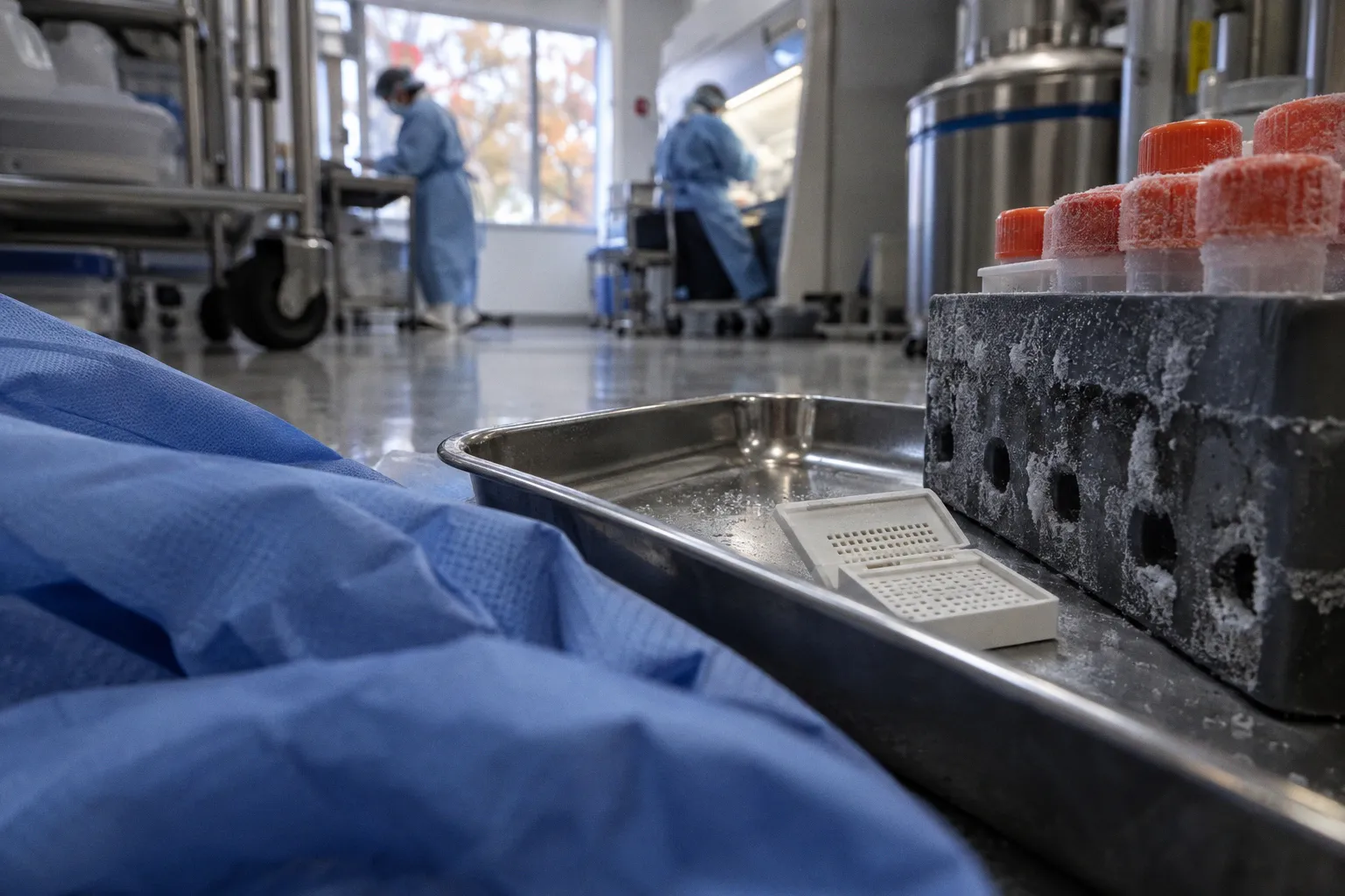
A retina held under uncontrolled conditions can lose photoreceptor metabolic capacity rapidly. A retina cooled early and maintained within a controlled 2°C–8°C chain can remain proteomically usable much longer than older procurement rules often imply.
Recent human donor-eye data extend the operational window for retinal multiomics. In a quantitative analysis of 6,109 retinal proteins, no statistically significant difference in protein abundance was observed between 12 and 18 hours post-mortem when ocular cooling to 2°C–8°C began within 8 hours of death. RNA sequencing produced a similar result at the transcript level: among 22,446 identified retinal transcripts, only five showed significant differential expression between the two intervals.
This does not make post-mortem delay irrelevant. It changes the problem from a simple clock threshold into a controlled logistics equation.
The 18-hour window is conditional, not universal
The most useful result is also the easiest to misapply. The 18-hour interval is not a general preservation guarantee. It is an observed stability window under defined cooling conditions.
The study compared donor retinas collected at 12 and 18 hours post-mortem. The tissue entered an early cold chain, with cooling to 2°C–8°C within 8 hours of death. Under those conditions, the measured abundance of 6,109 proteins did not differ significantly between the two groups. Cell-type-specific retinal protein markers also remained stable. The same applied to molecular markers relevant to age-related macular degeneration and glaucoma.
That result has direct implications for donor eye procurement. A specimen arriving at an eye bank after 17 hours is not automatically unsuitable for proteomics. Its value depends on the preceding thermal history and on whether the timestamps are reliable.
The relevant variables are:
- time from death to authorization;
- time from death to ocular cooling;
- time from death to recovery;
- time from recovery to eye-bank check-in;
- temperature during every unmonitored transfer;
- tissue dissection and freezing latency after check-in;
- preservation of separate metadata for each eye and each tissue compartment.
A single post-mortem interval number compresses all of these variables into one field. That is convenient for database filtering. It is weak for quality control.
An 18-hour post-mortem interval is a valid operating window only when temperature control is part of the interval record.
The practical distinction is between chronological age and biological exposure. Two retinas can have the same death-to-recovery interval and materially different molecular quality if one was cooled early and the other remained at uncontrolled temperature.
Why the 8-hour cooling boundary matters
The available data support cooling to 2°C–8°C within 8 hours of death as the critical operational condition. This does not mean that molecular change begins exactly at hour eight. Biological degradation is continuous. The boundary is a workflow requirement that separates a documented cold-chain specimen from an uncertain one.
For a research database, the field should not be recorded as a binary label such as cooled or not cooled. A more useful record captures:
1. death timestamp, with source and precision;
2. authorization timestamp;
3. first cooling timestamp;
4. cooling method and storage range;
5. recovery timestamp;
6. eye-bank receipt timestamp;
7. dissection timestamp;
8. snap-freezing or other terminal preservation timestamp.
Without this sequence, downstream users cannot distinguish a robust 18-hour specimen from a nominally similar sample that spent several hours at ambient conditions.
Cold-chain dynamics determine the degradation curve
Human retinas are not inert material after death. Their molecular state changes as oxygen delivery stops, energy stores are depleted, and cellular maintenance processes fail. The speed of this transition is temperature-dependent.
In uncooled post-mortem conditions between 2 and 4.5 hours after death, photoreceptor metabolic processes decline linearly at approximately 16% to 19% per hour. This is not a direct measurement of total retinal protein loss. It is a measure of decline in photoreceptor metabolic capacity. The distinction matters. A falling metabolic signal does not mean that every protein has degraded at the same rate, or that bulk protein abundance has collapsed.
It does establish the cost of uncontrolled delay. The early period is not a harmless buffer before the cold chain begins. Photoreceptors have high metabolic demand and are especially sensitive to interruption of energy homeostasis. Their functional decline can precede obvious bulk-proteome changes.
This creates two separate quality dimensions:
- structural or bulk proteomic stability, assessed through protein abundance and marker preservation;
- functional and cell-state integrity, assessed through metabolic pathways, transcript patterns, and cell-type-specific signals.
A specimen can remain acceptable for a particular bulk proteomics assay while carrying altered signatures in vulnerable cell populations. Conversely, a modest change in a metabolic pathway may not invalidate a study focused on stable structural proteins.
Temperature is a metadata variable, not a storage footnote
Cold-chain documentation should be treated as part of the biospecimen itself. A proteomics dataset without temperature history has a missing explanatory variable.
At minimum, procurement systems should distinguish:
| Variable | Controlled specimen | Uncertain specimen |
|---|---|---|
| Initial cooling | Documented start within the defined workflow | Missing or estimated |
| Storage range | Maintained at 2°C–8°C | Ambient exposure or unknown range |
| Death-to-recovery interval | Timestamped | Rounded or reconstructed |
| Tissue condition at intake | Linked to inspection record | Described without timestamp |
| Multiomics interpretation | Eligible for interval-based comparison | Requires conservative stratification |
| Database use | Suitable for controlled cohort design | Suitable only with explicit quality flags |
The key failure mode is not necessarily late recovery. It is late recovery with no thermal trace.
For procurement teams, this means that the first operational target should be cooling latency, not simply reducing the final death-to-check-in interval. A shorter administrative process is useful. It does not compensate for an uncontrolled first phase.
What the proteomic data actually show
The retinal proteomic analysis used 16-plex TMT mass spectrometry and quantified 6,109 proteins. The central finding was the absence of statistically significant differences in protein abundance between 12-hour and 18-hour post-mortem groups under early ocular cooling.
This is a strong result for cohort design. It suggests that the additional six hours do not automatically introduce a large bulk-proteome shift when the cold chain is maintained. It also supports the inclusion of donor retinas across a broader interval range, provided that the interval and cooling variables are modeled rather than ignored.
The result does not establish a retinal protein half-life post-mortem. Half-life requires a defined decay model, repeated measurements across a time series, and sufficient resolution to estimate the kinetics of individual proteins or protein classes. A comparison between two time points can demonstrate stability within that range. It cannot produce a universal degradation constant.
The same limitation applies to the phrase protein degradation rate. There is no single rate for the human retina. Kinetics vary according to:
- protein localization;
- turnover before death;
- association with membranes or organelles;
- protease susceptibility;
- phosphorylation or other modification state;
- cell-type distribution;
- tissue handling after recovery;
- freeze-thaw exposure;
- extraction and digestion protocol.
A stable bulk abundance measurement can conceal changes in isoforms, cleavage products, post-translational modifications, or rare cell populations. The study therefore supports a bounded operational conclusion: under early cooling, bulk retinal protein abundance and disease-relevant markers remain stable between 12 and 18 hours. It does not support an unrestricted claim of molecular preservation across all analytes.
Disease markers remain usable within the tested range
The stability of molecular markers associated with age-related macular degeneration and glaucoma is important for translational studies. Donor tissue procurement frequently produces cohorts with unavoidable variation in recovery timing. If every interval beyond 12 hours were treated as molecularly compromised, cohort size would shrink and selection bias would increase.
The data indicate that properly cooled specimens up to 18 hours can remain compatible with disease-focused protein analysis. This is particularly relevant when the study requires both diseased and control eyes. Excluding all longer-interval tissue may create an imbalanced cohort if disease status, age, cause of death, or geography is correlated with recovery logistics.
However, interval matching remains necessary. A glaucoma cohort collected primarily at 17–18 hours should not be compared with controls collected at 6–8 hours without adjustment. The absence of a significant difference between 12 and 18 hours in one controlled analysis is not permission to disregard all pre-analytic variation.
A practical cohort model should retain post-mortem interval as a continuous variable where sample size permits. If the dataset is smaller, interval bins can be used, but the bins should preserve the operational distinction between:
- early cooled tissue;
- late cooled tissue;
- documented cold-chain tissue;
- unknown thermal history.
These categories carry more information than a single pass/fail label.
Transcriptomic resilience does not erase cell-state effects
RNA sequencing identified 22,446 retinal transcripts. Only five showed significant differential expression between the 12-hour and 18-hour groups under the same early-cooling conditions.
This is a narrow transcriptomic shift across the tested interval. It supports the view that controlled cooling can preserve a substantial portion of the retinal molecular profile through 18 hours. It also provides a useful counterweight to overly conservative procurement rules that reject any tissue beyond a fixed 12-hour threshold.
But transcriptomic stability must be interpreted at the correct resolution.
Bulk RNA sequencing averages signals across photoreceptors, retinal ganglion cells, bipolar cells, amacrine cells, Müller glia, vascular components, and other tissue elements. A small or vulnerable cell population can undergo meaningful state changes without producing a large bulk-tissue signal. Single-cell RNA sequencing and spatial transcriptomics have different tolerance requirements because they depend on cell recovery, RNA integrity, dissociation behavior, and preservation of spatial architecture.
The study therefore provides stronger support for bulk transcriptomic comparison than for every possible single-cell workflow. It is reasonable to use the findings when planning donor retinal RNA-seq cohorts. It is less defensible to assume identical preservation for all cell-type-resolved applications.
The distinction between abundance and identity
Bulk RNA-seq and bulk proteomics answer different questions from cell-resolved assays.
A bulk assay asks whether the aggregate molecular composition of the tissue has changed enough to alter group-level analysis. A single-cell assay asks whether individual cell populations remain recoverable and biologically interpretable. The first can remain stable while the second loses sensitivity through selective cell damage or reduced recovery.
For donor-eye databases, this means sample annotations should include the intended assay class. A specimen may be:
- suitable for bulk proteomics;
- suitable for bulk RNA sequencing;
- conditionally suitable for targeted disease-marker analysis;
- uncertain for single-cell sequencing;
- unsuitable for assays requiring live-cell function.
These are not interchangeable labels. They should not be collapsed into a general designation such as high quality.
Procurement latency is the hidden constraint
The molecular findings are clear. The eye-bank workflow is less forgiving.
The average donor death-to-authorization time is 7.0 hours, with a median of 5.5 hours. Average death-to-recovery is 12.6 hours, with a median of 11.5 hours. Average death-to-eye-bank check-in is 17.0 hours, with a median of 15.8 hours.
These values show why the 18-hour window matters operationally. The average check-in time approaches the upper bound of the tested proteomic interval. A workflow that treats check-in as the beginning of quality assessment is already operating near the end of the molecularly characterized window.
The bottleneck is distributed across the system:
1. Authorization latency. Next-of-kin authorization can consume a large fraction of the early post-mortem period. This is an administrative variable, but it directly affects cooling and recovery timing.
2. Transport latency. The gap between authorization, recovery, and facility arrival can vary by geography, staffing, and transport availability.
3. Recovery scheduling. A donor may be eligible while the retrieval team is not immediately available.
4. Intake latency. Tissue can arrive at the eye bank but remain unprocessed while accessioning, inspection, and routing are completed.
5. Research allocation latency. The interval between check-in and dissection can be invisible if only death-to-recovery is recorded.
Each stage creates a separate timestamp requirement. The final post-mortem interval is a summary metric, not a process map.
The procurement system does not lose data quality at one dramatic failure point. It loses it through accumulated latency between ordinary handoffs.
Building a usable donor-eye record
A multiomics-ready eye-bank database should be designed around event time, not only specimen identity. The record must allow researchers to reconstruct what happened before the tissue entered a freezer.
A minimum event model includes:
- donor death;
- authorization;
- first cooling;
- recovery start and completion;
- transport departure and arrival;
- eye-bank check-in;
- gross inspection;
- tissue dissection;
- aliquoting;
- preservation;
- freezer placement;
- downstream shipment.
Every event should have a timestamp, an operator or system origin, and a confidence flag where the time is estimated. Missingness also requires a code. An absent timestamp is not the same as a confirmed zero delay.
For data harmonization, the database should retain both raw timestamps and derived intervals. Derived fields are useful for analysis. Raw fields are required for auditability.
Recommended derived fields include:
- death-to-cooling;
- death-to-authorization;
- death-to-recovery;
- death-to-check-in;
- recovery-to-freezing;
- cumulative time outside the documented 2°C–8°C range;
- total number of temperature excursions;
- temperature-history completeness.
The last field is often neglected. A specimen with 16 hours in the cold chain and a specimen with 16 hours reported as cold but no monitoring record should not receive the same confidence score.
Designing cohorts around measured stability
A fixed exclusion threshold is easy to implement. It is also a crude model of tissue quality.
The current evidence supports a more granular approach. For bulk retinal proteomics, tissue collected between 12 and 18 hours can remain analytically useful when cooling begins within 8 hours and the 2°C–8°C chain is maintained. That interval should be available to researchers rather than automatically discarded.
The correct strategy is stratification. Cohorts can be grouped by interval and thermal control, then analyzed for residual pre-analytic effects. The analysis plan should specify whether post-mortem interval is:
- an inclusion criterion;
- a covariate;
- a matching variable;
- a sensitivity-analysis parameter;
- a reason for exclusion only when combined with missing thermal data.
For disease studies, group balance is important. If all control eyes are recovered rapidly but many disease eyes arrive later, post-mortem interval can become a confounder. If all older donors experience longer authorization latency, age and interval can become partially coupled. If a specific region has slower transport, geography can enter the molecular model indirectly.
This is why procurement metadata belongs beside sequencing and mass-spectrometry output. It is not administrative decoration. It is part of the explanatory architecture.
A practical classification for research release
A database can make this logic operational by assigning tissue to quality tiers based on documented events.
Tier 1: controlled interval. Cooling begins within the defined early window, storage remains at 2°C–8°C, and recovery, check-in, and preservation times are recorded.
Tier 2: acceptable interval with partial documentation. The reported interval falls within the tested range, but one part of the thermal or handling history is incomplete.
Tier 3: extended or uncertain interval. The specimen may still be useful, but the dataset requires explicit adjustment, validation, or assay-specific review.
Tier 4: uncontrolled exposure. Ambient storage, prolonged temperature uncertainty, or major timestamp gaps prevent confident interpretation of degradation-sensitive assays.
These tiers should not be presented as universal biological truths. They are data-governance tools. Their value comes from making uncertainty visible before the tissue is selected for a study.
Implications for mass spectrometry quality control
Mass spectrometry ocular tissue quality control should combine molecular readouts with procurement metadata. Instrument-level metrics cannot recover a specimen from an undocumented pre-analytic failure.
For retinal proteomics, the QC layer should assess:
- peptide and protein identification depth;
- missingness across samples;
- technical replicate agreement;
- batch-associated variance;
- abundance of cell-type-specific markers;
- abundance of disease-relevant markers;
- evidence of proteolytic fragmentation where the assay can detect it;
- association between molecular output and post-mortem interval;
- association between molecular output and temperature-history completeness.
The 6,109-protein result provides a benchmark for what stability can look like under controlled conditions. It should not be converted into a universal expected identification count for every laboratory. Instrument platform, sample preparation, tissue region, extraction method, and database search strategy will alter coverage.
Similarly, the absence of significant abundance differences between 12 and 18 hours does not mean that every individual protein is unchanged. Statistical stability at the cohort level can coexist with local effects, low-abundance shifts, or modifications outside the assay’s measurement range.
A rigorous release pipeline should therefore include both global and targeted QC. Global metrics identify broad degradation or batch failure. Targeted markers test whether retinal cell composition and disease-relevant biology remain interpretable.
What remains unknown beyond 18 hours
The evidence establishes a useful 12-to-18-hour comparison. It does not define the full degradation trajectory beyond that range.
Long-term proteomic decay rates for human retinas preserved beyond 24 hours without flash-freezing remain unresolved in the available evidence. Cell-type-resolved degradation profiles for rare retinal populations, including specific amacrine or bipolar subtypes, are also not established beyond the bulk-tissue measurements.
This limits how far procurement policies can be generalized. A sample at 20 or 24 hours may still produce valuable data. It cannot be assigned the same evidence-backed status as a properly cooled 18-hour sample solely because the storage temperature appears acceptable.
The same caution applies to tissue compartments. Retina, retinal pigment epithelium, choroid, optic nerve, and other ocular tissues have different cellular compositions and metabolic characteristics. Stability data from bulk human retina should not be transferred automatically to choroid gene-expression profiling or optic-nerve proteomics.
Assay scope also matters. A tissue that remains adequate for bulk protein abundance analysis may not be adequate for:
- labile post-translational modification measurements;
- spatial molecular profiling;
- high-resolution single-cell analysis;
- functional assays requiring viable cells;
- analyses of rapidly changing metabolic intermediates.
A donor-eye catalogue should expose these boundaries. It should not imply that one stability interval applies to all ocular multiomics.
The operational standard
The evidence supports a clear procurement position.
First, early cooling is the primary controllable intervention. It should begin as soon as the workflow permits and be documented with a timestamp. Second, the 2°C–8°C chain should be maintained and monitored rather than inferred from standard operating procedure. Third, death-to-recovery and death-to-check-in should remain separate fields. Fourth, researchers should receive the full interval history instead of a single quality label. Fifth, the 12-to-18-hour window should be treated as conditionally usable for bulk retinal proteomics and transcriptomics, not as a universal pass threshold for every assay.
The practical consequence is a change in prioritization. Eye banks and research coordinators do not need to pursue a single headline metric while ignoring the rest of the pipeline. They need to reduce cooling latency, preserve event-level metadata, and prevent temperature uncertainty from being hidden inside an apparently acceptable post-mortem interval.
Post-mortem retinal protein degradation rates are therefore best managed as a systems problem. The current proteomic and transcriptomic data show that controlled cooling can preserve retinal molecular integrity through 18 hours under defined conditions. They do not justify extending that window without qualification, and they do not eliminate the need for assay-specific quality control.
For ocular multiomics, the strongest specimen is not simply the one recovered fastest. It is the one whose biological history is measured, timestamped, temperature-controlled, and available to the analyst.